Continuous Wavelet Transform (CWT)

This section describes functions used to perform single continuous wavelet transforms.

Single level - cwt

pywt.cwt(data, scales, wavelet)

One dimensional Continuous Wavelet Transform.

Parameters:

data : array_like

Input signal

scales : array_like

The wavelet scales to use. One can use f = scale2frequency(wavelet, scale)/sampling_period to determine what physical frequency, f. Here, f is in hertz when the sampling_period is given in seconds.

wavelet : Wavelet object or name

Wavelet to use

sampling_period : float

Sampling period for the frequencies output (optional). The values computed for coefs are independent of the choice of sampling_period (i.e. scales is not scaled by the sampling period).

method : {‘conv’, ‘fft’}, optional

The method used to compute the CWT. Can be any of:

• conv uses numpy.convolve.
• fft uses frequency domain convolution.
• auto uses automatic selection based on an estimate of the computational complexity at each scale.

The conv method complexity is O(len(scale) * len(data)). The fft method is O(N * log2(N)) with N = len(scale) + len(data) - 1. It is well suited for large size signals but slightly slower than conv on small ones.

axis: int, optional

Axis over which to compute the CWT. If not given, the last axis is used.

Returns:

coefs : array_like

Continuous wavelet transform of the input signal for the given scales and wavelet. The first axis of coefs corresponds to the scales. The remaining axes match the shape of data.

frequencies : array_like

If the unit of sampling period are seconds and given, than frequencies are in hertz. Otherwise, a sampling period of 1 is assumed.

Notes

Size of coefficients arrays depends on the length of the input array and the length of given scales.

Examples

>>> import pywt
>>> import numpy as np
>>> import matplotlib.pyplot as plt
>>> x = np.arange(512)
>>> y = np.sin(2*np.pi*x/32)
>>> coef, freqs=pywt.cwt(y,np.arange(1,129),'gaus1')
>>> plt.matshow(coef) # doctest: +SKIP
>>> plt.show() # doctest: +SKIP
----------
>>> import pywt
>>> import numpy as np
>>> import matplotlib.pyplot as plt
>>> t = np.linspace(-1, 1, 200, endpoint=False)
>>> sig  = np.cos(2 * np.pi * 7 * t) + np.real(np.exp(-7*(t-0.4)**2)*np.exp(1j*2*np.pi*2*(t-0.4)))
>>> widths = np.arange(1, 31)
>>> cwtmatr, freqs = pywt.cwt(sig, widths, 'mexh')
>>> plt.imshow(cwtmatr, extent=[-1, 1, 1, 31], cmap='PRGn', aspect='auto',
...            vmax=abs(cwtmatr).max(), vmin=-abs(cwtmatr).max())  # doctest: +SKIP
>>> plt.show() # doctest: +SKIP

Continuous Wavelet Families

A variety of continuous wavelets have been implemented. A list of the available wavelet names compatible with cwt can be obtained by:

wavlist = pywt.wavelist(kind='continuous')

Mexican Hat Wavelet

The mexican hat wavelet "mexh" is given by:

\[\psi(t) = \frac{2}{\sqrt{3} \sqrt[4]{\pi}} \exp^{-\frac{t^2}{2}} \left( 1 - t^2 \right)\]

where the constant out front is a normalization factor so that the wavelet has unit energy.

Morlet Wavelet

The Morlet wavelet "morl" is given by:

\[\psi(t) = \exp^{-\frac{t^2}{2}} \cos(5t)\]

Complex Morlet Wavelets

The complex Morlet wavelet ("cmorB-C" with floating point values B, C) is given by:

\[\psi(t) = \frac{1}{\sqrt{\pi B}} \exp^{-\frac{t^2}{B}} \exp^{\mathrm{j} 2\pi C t}\]

where \(B\) is the bandwidth and \(C\) is the center frequency.

Gaussian Derivative Wavelets

The Gaussian wavelets ("gausP" where P is an integer between 1 and and 8) correspond to the Pth order derivatives of the function:

\[\psi(t) = C \exp^{-t^2}\]

where \(C\) is an order-dependent normalization constant.

Complex Gaussian Derivative Wavelets

The complex Gaussian wavelets ("cgauP" where P is an integer between 1 and 8) correspond to the Pth order derivatives of the function:

\[\psi(t) = C \exp^{-\mathrm{j} t}\exp^{-t^2}\]

where \(C\) is an order-dependent normalization constant.

Shannon Wavelets

The Shannon wavelets ("shanB-C" with floating point values B and C) correspond to the following wavelets:

\[\psi(t) = \sqrt{B} \frac{\sin(\pi B t)}{\pi B t} \exp^{\mathrm{j}2 \pi C t}\]

where \(B\) is the bandwidth and \(C\) is the center frequency.

Frequency B-Spline Wavelets

The frequency B-spline wavelets ("fpspM-B-C" with integer M and floating point B, C) correspond to the following wavelets:

\[\psi(t) = \sqrt{B} \left[\frac{\sin(\pi B \frac{t}{M})}{\pi B \frac{t}{M}}\right]^M \exp^{2\mathrm{j} \pi C t}\]

where \(M\) is the spline order, \(B\) is the bandwidth and \(C\) is the center frequency.

Choosing the scales for cwt

For each of the wavelets described below, the implementation in PyWavelets evaluates the wavelet function for \(t\) over the range [wavelet.lower_bound, wavelet.upper_bound] (with default range \([-8, 8]\)). scale = 1 corresponds to the case where the extent of the wavelet is (wavelet.upper_bound - wavelet.lower_bound + 1) samples of the digital signal being analyzed. Larger scales correspond to stretching of the wavelet. For example, at scale=10 the wavelet is stretched by a factor of 10, making it sensitive to lower frequencies in the signal.

To relate a given scale to a specific signal frequency, the sampling period of the signal must be known. pywt.scale2frequency() can be used to convert a list of scales to their corresponding frequencies. The proper choice of scales depends on the chosen wavelet, so pywt.scale2frequency() should be used to get an idea of an appropriate range for the signal of interest.

For the cmor, fbsp and shan wavelets, the user can specify a specific a normalized center frequency. A value of 1.0 corresponds to 1/dt where dt is the sampling period. In other words, when analyzing a signal sampled at 100 Hz, a center frequency of 1.0 corresponds to ~100 Hz at scale = 1. This is above the Nyquist rate of 50 Hz, so for this particular wavelet, one would analyze a signal using scales >= 2.

>>> import numpy as np
>>> import pywt
>>> dt = 0.01  # 100 Hz sampling
>>> frequencies = pywt.scale2frequency('cmor1.5-1.0', [1, 2, 3, 4]) / dt
>>> frequencies
array([ 100.        ,   50.        ,   33.33333333,   25.        ])

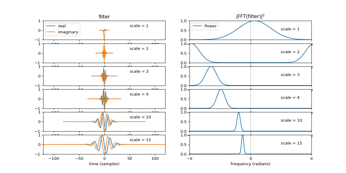
The CWT in PyWavelets is applied to discrete data by convolution with samples of the integral of the wavelet. If scale is too low, this will result in a discrete filter that is inadequately sampled leading to aliasing as shown in the example below. Here the wavelet is 'cmor1.5-1.0'. The left column of the figure shows the discrete filters used in the convolution at various scales. The right column are the corresponding Fourier power spectra of each filter.. For scales 1 and 2 it can be seen that aliasing due to violation of the Nyquist limit occurs.

import numpy as np
import pywt
import matplotlib.pyplot as plt

wav = pywt.ContinuousWavelet('cmor1.5-1.0')

# print the range over which the wavelet will be evaluated
print("Continuous wavelet will be evaluated over the range [{}, {}]".format(
    wav.lower_bound, wav.upper_bound))

width = wav.upper_bound - wav.lower_bound

scales = [1, 2, 3, 4, 10, 15]

max_len = int(np.max(scales)*width + 1)
t = np.arange(max_len)
fig, axes = plt.subplots(len(scales), 2, figsize=(12, 6))
for n, scale in enumerate(scales):

    # The following code is adapted from the internals of cwt
    int_psi, x = pywt.integrate_wavelet(wav, precision=10)
    step = x[1] - x[0]
    j = np.floor(
        np.arange(scale * width + 1) / (scale * step))
    if np.max(j) >= np.size(int_psi):
        j = np.delete(j, np.where((j >= np.size(int_psi)))[0])
    j = j.astype(np.int)

    # normalize int_psi for easier plotting
    int_psi /= np.abs(int_psi).max()

    # discrete samples of the integrated wavelet
    filt = int_psi[j][::-1]

    # The CWT consists of convolution of filt with the signal at this scale
    # Here we plot this discrete convolution kernel at each scale.

    nt = len(filt)
    t = np.linspace(-nt//2, nt//2, nt)
    axes[n, 0].plot(t, filt.real, t, filt.imag)
    axes[n, 0].set_xlim([-max_len//2, max_len//2])
    axes[n, 0].set_ylim([-1, 1])
    axes[n, 0].text(50, 0.35, 'scale = {}'.format(scale))

    f = np.linspace(-np.pi, np.pi, max_len)
    filt_fft = np.fft.fftshift(np.fft.fft(filt, n=max_len))
    filt_fft /= np.abs(filt_fft).max()
    axes[n, 1].plot(f, np.abs(filt_fft)**2)
    axes[n, 1].set_xlim([-np.pi, np.pi])
    axes[n, 1].set_ylim([0, 1])
    axes[n, 1].set_xticks([-np.pi, 0, np.pi])
    axes[n, 1].set_xticklabels([r'$-\pi$', '0', r'$\pi$'])
    axes[n, 1].grid(True, axis='x')
    axes[n, 1].text(np.pi/2, 0.5, 'scale = {}'.format(scale))

axes[n, 0].set_xlabel('time (samples)')
axes[n, 1].set_xlabel('frequency (radians)')
axes[0, 0].legend(['real', 'imaginary'], loc='upper left')
axes[0, 1].legend(['Power'], loc='upper left')
axes[0, 0].set_title('filter')
axes[0, 1].set_title(r'|FFT(filter)|$^2$')