Overview of multilevel wavelet decompositions

There are a number of different ways a wavelet decomposition can be performed for multiresolution analysis of n-dimensional data. Here we will review the three approaches currently implemented in PyWavelets. 2D cases are illustrated, but each of the approaches extends to the n-dimensional case in a straightforward manner.

Multilevel Discrete Wavelet Transform

The most common approach to the multilevel discrete wavelet transform involves further decomposition of only the approximation subband at each subsequent level. This is also sometimes referred to as the Mallat decomposition [Mall89]. In 2D, the discrete wavelet transform produces four sets of coefficients corresponding to the four possible combinations of the wavelet decomposition filters over the two separate axes. (In n-dimensions, there are 2**n sets of coefficients). For subsequent levels of decomposition, only the approximation coefficients (the lowpass subband) are further decomposed.

In PyWavelets, this decomposition is implemented for n-dimensional data by wavedecn() and the inverse by waverecn(). 1D and 2D versions of these routines also exist. It is illustrated in the figure below. The top row indicates the coefficient names as used by wavedec2() after each level of decomposition. The bottom row shows wavelet coefficients for the cameraman image (with each subband independently normalized for easier visualization).

import numpy as np
from matplotlib import pyplot as plt

import pywt
from pywt._doc_utils import draw_2d_wp_basis, wavedec2_keys

x = pywt.data.camera().astype(np.float32)
shape = x.shape

max_lev = 3       # how many levels of decomposition to draw
label_levels = 3  # how many levels to explicitly label on the plots

fig, axes = plt.subplots(2, 4, figsize=[14, 8])
for level in range(max_lev + 1):
    if level == 0:
        # show the original image before decomposition
        axes[0, 0].set_axis_off()
        axes[1, 0].imshow(x, cmap=plt.cm.gray)
        axes[1, 0].set_title('Image')
        axes[1, 0].set_axis_off()
        continue

    # plot subband boundaries of a standard DWT basis
    draw_2d_wp_basis(shape, wavedec2_keys(level), ax=axes[0, level],
                     label_levels=label_levels)
    axes[0, level].set_title(f'{level} level\ndecomposition')

    # compute the 2D DWT
    c = pywt.wavedec2(x, 'db2', mode='periodization', level=level)
    # normalize each coefficient array independently for better visibility
    c[0] /= np.abs(c[0]).max()
    for detail_level in range(level):
        c[detail_level + 1] = [d/np.abs(d).max() for d in c[detail_level + 1]]
    # show the normalized coefficients
    arr, slices = pywt.coeffs_to_array(c)
    axes[1, level].imshow(arr, cmap=plt.cm.gray)
    axes[1, level].set_title(f'Coefficients\n({level} level)')
    axes[1, level].set_axis_off()

plt.tight_layout()
plt.show()

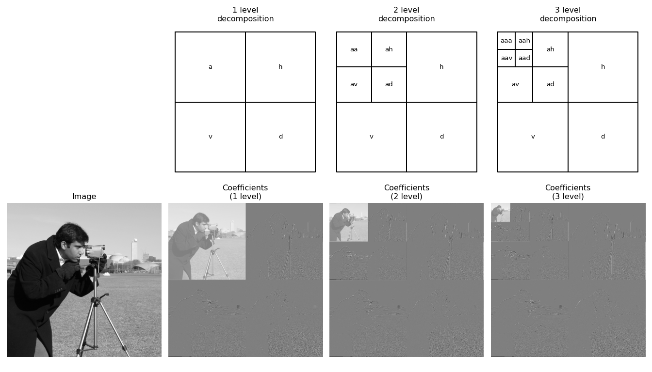
It can be seen that many of the coefficients are near zero (gray). This ability of the wavelet transform to sparsely represent natural images is a key property that makes it desirable in applications such as image compression and restoration.

Fully Separable Discrete Wavelet Transform

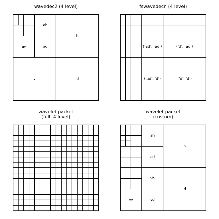
An alternative decomposition results in first fully decomposing one axis of the data prior to moving onto each additional axis in turn. This is illustrated for the 2D case in the upper right panel of the figure below. This approach has a factor of two higher computational cost as compared to the Mallat approach, but has advantages in compactly representing anisotropic data. A demo of this is available).

This form of the DWT is also sometimes referred to as the tensor wavelet transform or the hyperbolic wavelet transform. In PyWavelets it is implemented for n-dimensional data by fswavedecn() and the inverse by fswaverecn().

Wavelet Packet Transform

Another possible choice is to apply additional levels of decomposition to all wavelet subbands from the first level as opposed to only the approximation subband. This is known as the wavelet packet transform and is illustrated in 2D in the lower left panel of the figure. It is also possible to only perform any subset of the decompositions, resulting in a wide number of potential wavelet packet bases. An arbitrary example is shown in the lower right panel of the figure below.

A further description is available in the wavelet packet documentation.

For the wavelet packets, the plots below use “natural” ordering for simplicity, but this does not directly match the “frequency” ordering for these wavelet packets. It is possible to rearrange the coefficients into frequency ordering (see the get_level method of WaveletPacket2D and [Wick94] for more details).

from itertools import product

import numpy as np
from matplotlib import pyplot as plt

from pywt._doc_utils import (
    draw_2d_fswavedecn_basis,
    draw_2d_wp_basis,
    wavedec2_keys,
    wavedec_keys,
)

shape = (512, 512)

max_lev = 4       # how many levels of decomposition to draw
label_levels = 2  # how many levels to explicitly label on the plots

if False:
    fig, axes = plt.subplots(1, 4, figsize=[16, 4])
    axes = axes.ravel()
else:
    fig, axes = plt.subplots(2, 2, figsize=[8, 8])
    axes = axes.ravel()

# plot a 5-level standard DWT basis
draw_2d_wp_basis(shape, wavedec2_keys(max_lev), ax=axes[0],
                 label_levels=label_levels)
axes[0].set_title(f'wavedec2 ({max_lev} level)')

# plot for the fully separable case
draw_2d_fswavedecn_basis(shape, max_lev, ax=axes[1], label_levels=label_levels)
axes[1].set_title(f'fswavedecn ({max_lev} level)')

# get all keys corresponding to a full wavelet packet decomposition
wp_keys = list(product(['a', 'd', 'h', 'v'], repeat=max_lev))
draw_2d_wp_basis(shape, wp_keys, ax=axes[2])
axes[2].set_title(f'wavelet packet\n(full: {max_lev} level)')

# plot an example of a custom wavelet packet basis
keys = ['aaaa', 'aaad', 'aaah', 'aaav', 'aad', 'aah', 'aava', 'aavd',
        'aavh', 'aavv', 'ad', 'ah', 'ava', 'avd', 'avh', 'avv', 'd', 'h',
        'vaa', 'vad', 'vah', 'vav', 'vd', 'vh', 'vv']
draw_2d_wp_basis(shape, keys, ax=axes[3], label_levels=label_levels)
axes[3].set_title('wavelet packet\n(custom)')

plt.tight_layout()
plt.show()

References

Mall89

Mallat, S.G. “A Theory for Multiresolution Signal Decomposition: The Wavelet Representation” IEEE Transactions on Pattern Analysis and Machine Intelligence, vol. 2, no. 7. July 1989. DOI: 10.1109/34.192463

Wick94

Wickerhauser, M.V. “Adapted Wavelet Analysis from Theory to Software” Wellesley. Massachusetts: A K Peters. 1994.