Continuous Wavelet Transform (CWT)#
This section focuses on the one-dimensional Continuous Wavelet Transform. It
introduces the main function cwt alongside several helper function, and
also gives an overview over the available wavelets for this transfom.
Note
cwt and related functions in PyWavelets have some known issues;
you may be interested in trying the cwt implementation in
ssqueezepy,
which is substantially faster and may also be more accurate.
Introduction#
In simple terms, the Continuous Wavelet Transform is an analysis tool similar to the Fourier Transform, in that it takes a time-domain signal and returns the signal’s components in the frequency domain. However, in contrast to the Fourier Transform, the Continuous Wavelet Transform returns a two-dimensional result, providing information in the frequency- as well as in time-domain. Therefore, it is useful for periodic signals which change over time, such as audio, seismic signals and many others (see below for examples).
For more background and an in-depth guide to the application of the Continuous Wavelet Transform, including topics such as statistical significance, the following well-known article is highly recommended:
The cwt Function#
This is the main function, which calculates the Continuous Wavelet Transform of a one-dimensional signal.
- pywt.cwt(data, scales, wavelet, sampling_period=1.0, method='conv', axis=-1, *, precision=12)#
One dimensional Continuous Wavelet Transform.
- Parameters:
- dataarray_like
Input signal
- scalesarray_like
The wavelet scales to use. One can use
f = scale2frequency(wavelet, scale)/sampling_periodto determine what physical frequency,f. Here,fis in hertz when thesampling_periodis given in seconds.- waveletWavelet object or name
Wavelet to use
- sampling_periodfloat
Sampling period for the frequencies output (optional). The values computed for
coefsare independent of the choice ofsampling_period(i.e.scalesis not scaled by the sampling period).- method{‘conv’, ‘fft’}, optional
- The method used to compute the CWT. Can be any of:
convusesnumpy.convolve.fftuses frequency domain convolution.autouses automatic selection based on an estimate of the computational complexity at each scale.
The
convmethod complexity isO(len(scale) * len(data)). Thefftmethod isO(N * log2(N))withN = len(scale) + len(data) - 1. It is well suited for large size signals but slightly slower thanconvon small ones.- axis: int, optional
Axis over which to compute the CWT. If not given, the last axis is used.
- precision: int, optional
Length of wavelet (
2 ** precision) used to compute the CWT. Greater will increase resolution, especially for higher scales, but will compute a bit slower. Too low will distort coefficients and their norms, with a zipper-like effect. The default is 12, it’s recommended to use >=12.
- Returns:
- coefsarray_like
Continuous wavelet transform of the input signal for the given scales and wavelet. The first axis of
coefscorresponds to the scales. The remaining axes match the shape ofdata.- frequenciesarray_like
If the unit of sampling period are seconds and given, then frequencies are in hertz. Otherwise, a sampling period of 1 is assumed.
Notes
Size of coefficients arrays depends on the length of the input array and the length of given scales.
Examples
>>> import pywt
>>> import numpy as np
>>> import matplotlib.pyplot as plt
>>> x = np.exp(np.linspace(0, 2, 512))
>>> y = np.cos(2*np.pi*x)  # exponential chirp
>>> scales = np.logspace(np.log10(1), np.log10(128), 128)
>>> coef, freqs = pywt.cwt(y, scales, 'gaus1')
>>> plt.matshow(coef)
>>> plt.show()
>>> import pywt
>>> import numpy as np
>>> import matplotlib.pyplot as plt
>>> t = np.linspace(-1, 1, 200, endpoint=False)
>>> sig  = np.cos(2 * np.pi * 7 * t) + np.real(np.exp(-7*(t-0.4)**2)*np.exp(1j*2*np.pi*2*(t-0.4)))
>>> widths = np.logspace(np.log10(1), np.log10(30), 30)
>>> cwtmatr, freqs = pywt.cwt(sig, widths, 'mexh')
>>> plt.imshow(cwtmatr, extent=[-1, 1, 1, 31], cmap='PRGn', aspect='auto',
...            vmax=abs(cwtmatr).max(), vmin=-abs(cwtmatr).max())
>>> plt.show()
A comprehensive example of the CWT#
Here is a simple end-to-end example of how to calculate the CWT of a simple
signal, and how to plot it using matplotlib.
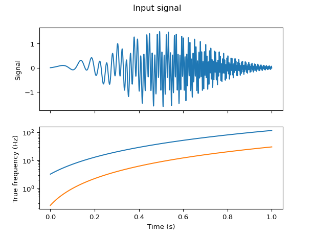
First, we generate an artificial signal to be analyzed. We are using the sum of two sine functions with increasing frequency, known as “chirp”. For reference, we also generate a plot of the signal and the two time-dependent frequency components it contains.
We then apply the Continuous Wavelet Transform
using a complex Morlet wavlet with a given center frequency and bandwidth
(namely cmor1.5-1.0). We then plot the so-called “scaleogram”, which is the
2D plot of the signal strength vs. time and frequency.
import matplotlib.pyplot as plt
import numpy as np

import pywt


def gaussian(x, x0, sigma):
    return np.exp(-np.power((x - x0) / sigma, 2.0) / 2.0)


def make_chirp(t, t0, a):
    frequency = (a * (t + t0)) ** 2
    chirp = np.sin(2 * np.pi * frequency * t)
    return chirp, frequency


# generate signal
time = np.linspace(0, 1, 2000)
chirp1, frequency1 = make_chirp(time, 0.2, 9)
chirp2, frequency2 = make_chirp(time, 0.1, 5)
chirp = chirp1 + 0.6 * chirp2
chirp *= gaussian(time, 0.5, 0.2)

# plot signal
fig, axs = plt.subplots(2, 1, sharex=True)
axs[0].plot(time, chirp)
axs[1].plot(time, frequency1)
axs[1].plot(time, frequency2)
axs[1].set_yscale("log")
axs[1].set_xlabel("Time (s)")
axs[0].set_ylabel("Signal")
axs[1].set_ylabel("True frequency (Hz)")
plt.suptitle("Input signal")
plt.show()
# perform CWT
wavelet = "cmor1.5-1.0"
# logarithmic scale for scales, as suggested by Torrence & Compo:
widths = np.geomspace(1, 1024, num=100)
sampling_period = np.diff(time).mean()
cwtmatr, freqs = pywt.cwt(chirp, widths, wavelet, sampling_period=sampling_period)
# absolute take absolute value of complex result
cwtmatr = np.abs(cwtmatr[:-1, :-1])

# plot result using matplotlib's pcolormesh (image with annoted axes)
fig, axs = plt.subplots(2, 1)
pcm = axs[0].pcolormesh(time, freqs, cwtmatr)
axs[0].set_yscale("log")
axs[0].set_xlabel("Time (s)")
axs[0].set_ylabel("Frequency (Hz)")
axs[0].set_title("Continuous Wavelet Transform (Scaleogram)")
fig.colorbar(pcm, ax=axs[0])

# plot fourier transform for comparison
from numpy.fft import rfft, rfftfreq

yf = rfft(chirp)
xf = rfftfreq(len(chirp), sampling_period)
plt.semilogx(xf, np.abs(yf))
axs[1].set_xlabel("Frequency (Hz)")
axs[1].set_title("Fourier Transform")
plt.tight_layout()
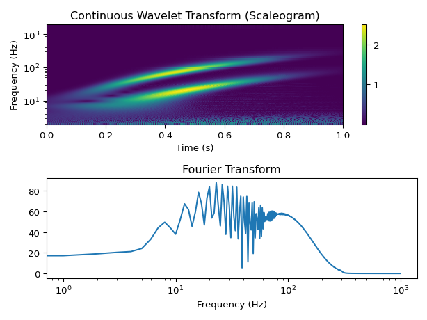
The Continuous Wavelet Transform can resolve the two frequency components clearly,
which is an obvious advantage over the Fourier Transform in this case. The scales
(widths) are given on a logarithmic scale in the example. The scales determine the
frequency resolution of the scaleogram. However, it is not straightforward to
convert them to frequencies, but luckily, cwt calculates the correct frequencies
for us. There are also helper functions, that perform this conversion in both ways.
For more information, see Choosing the scales for cwt and Converting frequency to scale for cwt.
Also note, that the raw output of cwt is complex if a complex wavelet is used.
For visualization, it is therefore necessary to use the absolute value.
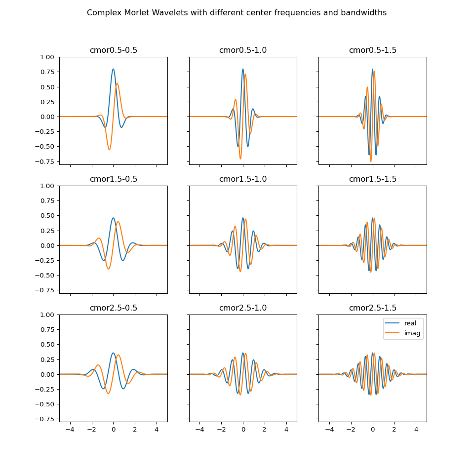
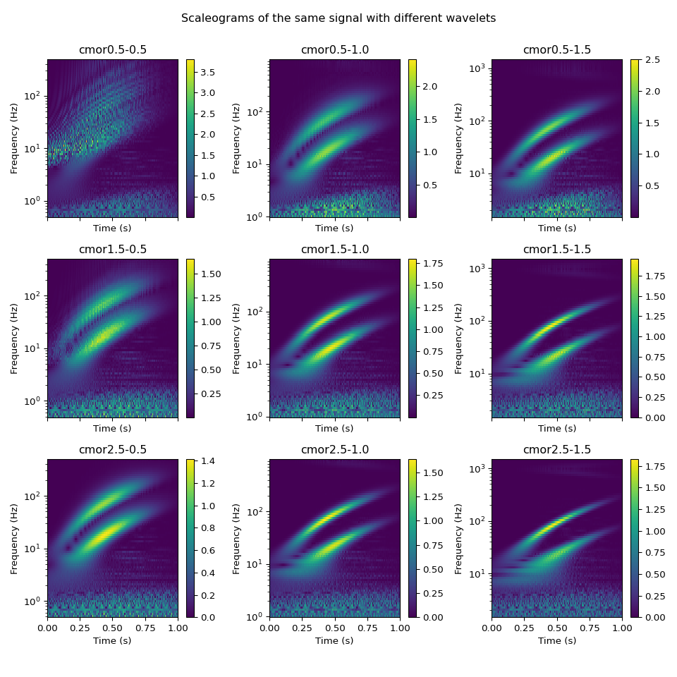
Wavelet bandwidth and center frequencies#
This example shows how the Complex Morlet Wavelet can be configured for optimum
results using the center_frequency and bandwidth_frequency parameters,
which can simply be appended to the wavelet’s string identifier cmor for
convenience. It also demonstrates the importance of choosing appropriate values
for the wavelet’s center frequency and bandwidth. The right values will depend
on the signal being analyzed. As shown below, bad values may lead to poor
resolution or artifacts.
import matplotlib.pyplot as plt
import numpy as np

import pywt

# plot complex morlet wavelets with different center frequencies and bandwidths
wavelets = [f"cmor{x:.1f}-{y:.1f}" for x in [0.5, 1.5, 2.5] for y in [0.5, 1.0, 1.5]]
fig, axs = plt.subplots(3, 3, figsize=(10, 10), sharex=True, sharey=True)
for ax, wavelet in zip(axs.flatten(), wavelets):
    [psi, x] = pywt.ContinuousWavelet(wavelet).wavefun(10)
    ax.plot(x, np.real(psi), label="real")
    ax.plot(x, np.imag(psi), label="imag")
    ax.set_title(wavelet)
    ax.set_xlim([-5, 5])
    ax.set_ylim([-0.8, 1])
ax.legend()
plt.suptitle("Complex Morlet Wavelets with different center frequencies and bandwidths")
plt.show()
def gaussian(x, x0, sigma):
    return np.exp(-np.power((x - x0) / sigma, 2.0) / 2.0)


def make_chirp(t, t0, a):
    frequency = (a * (t + t0)) ** 2
    chirp = np.sin(2 * np.pi * frequency * t)
    return chirp, frequency


def plot_wavelet(time, data, wavelet, title, ax):
    widths = np.geomspace(1, 1024, num=75)
    cwtmatr, freqs = pywt.cwt(
        data, widths, wavelet, sampling_period=np.diff(time).mean()
    )
    cwtmatr = np.abs(cwtmatr[:-1, :-1])
    pcm = ax.pcolormesh(time, freqs, cwtmatr)
    ax.set_yscale("log")
    ax.set_xlabel("Time (s)")
    ax.set_ylabel("Frequency (Hz)")
    ax.set_title(title)
    plt.colorbar(pcm, ax=ax)
    return ax


# generate signal
time = np.linspace(0, 1, 1000)
chirp1, frequency1 = make_chirp(time, 0.2, 9)
chirp2, frequency2 = make_chirp(time, 0.1, 5)
chirp = chirp1 + 0.6 * chirp2
chirp *= gaussian(time, 0.5, 0.2)

# perform CWT with different wavelets on same signal and plot results
wavelets = [f"cmor{x:.1f}-{y:.1f}" for x in [0.5, 1.5, 2.5] for y in [0.5, 1.0, 1.5]]
fig, axs = plt.subplots(3, 3, figsize=(10, 10), sharex=True)
for ax, wavelet in zip(axs.flatten(), wavelets):
    plot_wavelet(time, chirp, wavelet, wavelet, ax)
plt.tight_layout(rect=[0, 0.03, 1, 0.95])
plt.suptitle("Scaleograms of the same signal with different wavelets")
plt.show()
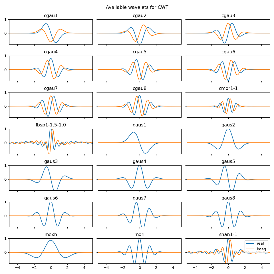
Continuous Wavelet Families#
A variety of continuous wavelets have been implemented. A list of the available
wavelet names compatible with cwt can be obtained by:
>>> import pywt
>>> wavelist = pywt.wavelist(kind='continuous')
Here is an overview of all available wavelets for cwt. Note, that they can be
customized by passing parameters such as center_frequency and bandwidth_frequency
(see ContinuousWavelet object for details).
import matplotlib.pyplot as plt
import numpy as np

import pywt

wavlist = pywt.wavelist(kind="continuous")
cols = 3
rows = (len(wavlist) + cols - 1) // cols
fig, axs = plt.subplots(rows, cols, figsize=(10, 10),
                        sharex=True, sharey=True)
for ax, wavelet in zip(axs.flatten(), wavlist):
    # A few wavelet families require parameters in the string name
    if wavelet in ['cmor', 'shan']:
        wavelet += '1-1'
    elif wavelet == 'fbsp':
        wavelet += '1-1.5-1.0'

    [psi, x] = pywt.ContinuousWavelet(wavelet).wavefun(10)
    ax.plot(x, np.real(psi), label="real")
    ax.plot(x, np.imag(psi), label="imag")
    ax.set_title(wavelet)
    ax.set_xlim([-5, 5])
    ax.set_ylim([-0.8, 1])

ax.legend(loc="upper right")
plt.suptitle("Available wavelets for CWT")
plt.tight_layout()
plt.show()
Mexican Hat Wavelet#
The mexican hat wavelet "mexh" is given by:
where the constant out front is a normalization factor so that the wavelet has unit energy.
Morlet Wavelet#
The Morlet wavelet "morl" is given by:
Complex Morlet Wavelets#
The complex Morlet wavelet ("cmorB-C" with floating point values B, C) is
given by:
where \(B\) is the bandwidth and \(C\) is the center frequency.
Gaussian Derivative Wavelets#
The Gaussian wavelets ("gausP" where P is an integer between 1 and and 8)
correspond to the Pth order derivatives of the function:
where \(C\) is an order-dependent normalization constant.
Complex Gaussian Derivative Wavelets#
The complex Gaussian wavelets ("cgauP" where P is an integer between 1 and
8) correspond to the Pth order derivatives of the function:
where \(C\) is an order-dependent normalization constant.
Shannon Wavelets#
The Shannon wavelets ("shanB-C" with floating point values B and C)
correspond to the following wavelets:
where \(B\) is the bandwidth and \(C\) is the center frequency.
Frequency B-Spline Wavelets#
The frequency B-spline wavelets ("fbspM-B-C" with integer M and floating
point B, C) correspond to the following wavelets:
where \(M\) is the spline order, \(B\) is the bandwidth and \(C\) is the center frequency.
Choosing the scales for cwt#
For each of the wavelets described below, the implementation in PyWavelets
evaluates the wavelet function for \(t\) over the range
[wavelet.lower_bound, wavelet.upper_bound] (with default range
\([-8, 8]\)). scale = 1 corresponds to the case where the extent of the
wavelet is (wavelet.upper_bound - wavelet.lower_bound + 1) samples of the
digital signal being analyzed. Larger scales correspond to stretching of the
wavelet. For example, at scale=10 the wavelet is stretched by a factor of
10, making it sensitive to lower frequencies in the signal.
To relate a given scale to a specific signal frequency, the sampling period
of the signal must be known. pywt.scale2frequency() can be used to
convert a list of scales to their corresponding frequencies. The proper choice
of scales depends on the chosen wavelet, so pywt.scale2frequency() should
be used to get an idea of an appropriate range for the signal of interest.
For the cmor, fbsp and shan wavelets, the user can specify a
specific a normalized center frequency. A value of 1.0 corresponds to 1/dt
where dt is the sampling period. In other words, when analyzing a signal
sampled at 100 Hz, a center frequency of 1.0 corresponds to ~100 Hz at
scale = 1. This is above the Nyquist rate of 50 Hz, so for this
particular wavelet, one would analyze a signal using scales >= 2.
>>> import numpy as np
>>> import pywt
>>> dt = 0.01  # 100 Hz sampling
>>> frequencies = pywt.scale2frequency('cmor1.5-1.0', [1, 2, 3, 4]) / dt
>>> frequencies
array([ 100.        ,   50.        ,   33.33333333,   25.        ])
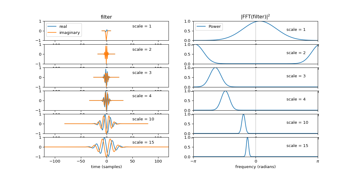
The CWT in PyWavelets is applied to discrete data by convolution with samples
of the integral of the wavelet. If scale is too low, this will result in
a discrete filter that is inadequately sampled leading to aliasing as shown
in the example below. Here the wavelet is 'cmor1.5-1.0'. The left column of
the figure shows the discrete filters used in the convolution at various
scales. The right column are the corresponding Fourier power spectra of each
filter.. For scales 1 and 2 it can be seen that aliasing due to violation of
the Nyquist limit occurs.
Converting frequency to scale for cwt#
To convert frequency to scale for use in the wavelet transform the function
pywt.frequency2scale() can be used. This is the complement of the
pywt.scale2frequency() function as seen in the previous section. Note that
the input frequency in this function is normalized by 1/dt, or the sampling
frequency fs. This function is useful for specifying the transform as a function
of frequency directly.
>>> import numpy as np
>>> import pywt
>>> dt = 0.01  # 100 Hz sampling
>>> fs = 1 / dt
>>> frequencies = np.array([100, 50, 33.33333333, 25]) / fs # normalize
>>> scale = pywt.frequency2scale('cmor1.5-1.0', frequencies)
>>> scale
array([ 1.,  2.,  3.,  4.])
import matplotlib.pyplot as plt
import numpy as np

import pywt

wav = pywt.ContinuousWavelet('cmor1.5-1.0')

# print the range over which the wavelet will be evaluated
print("Continuous wavelet will be evaluated over the range "
      f"[{wav.lower_bound}, {wav.upper_bound}]")

width = wav.upper_bound - wav.lower_bound

scales = [1, 2, 3, 4, 10, 15]

max_len = int(np.max(scales)*width + 1)
t = np.arange(max_len)
fig, axes = plt.subplots(len(scales), 2, figsize=(12, 6))
for n, scale in enumerate(scales):

    # The following code is adapted from the internals of cwt
    int_psi, x = pywt.integrate_wavelet(wav, precision=10)
    step = x[1] - x[0]
    j = np.floor(
        np.arange(scale * width + 1) / (scale * step))
    if np.max(j) >= np.size(int_psi):
        j = np.delete(j, np.where(j >= np.size(int_psi))[0])
    j = j.astype(np.int_)

    # normalize int_psi for easier plotting
    int_psi /= np.abs(int_psi).max()

    # discrete samples of the integrated wavelet
    filt = int_psi[j][::-1]

    # The CWT consists of convolution of filt with the signal at this scale
    # Here we plot this discrete convolution kernel at each scale.

    nt = len(filt)
    t = np.linspace(-nt//2, nt//2, nt)
    axes[n, 0].plot(t, filt.real, t, filt.imag)
    axes[n, 0].set_xlim([-max_len//2, max_len//2])
    axes[n, 0].set_ylim([-1, 1])
    axes[n, 0].text(50, 0.35, f'scale = {scale}')

    f = np.linspace(-np.pi, np.pi, max_len)
    filt_fft = np.fft.fftshift(np.fft.fft(filt, n=max_len))
    filt_fft /= np.abs(filt_fft).max()
    axes[n, 1].plot(f, np.abs(filt_fft)**2)
    axes[n, 1].set_xlim([-np.pi, np.pi])
    axes[n, 1].set_ylim([0, 1])
    axes[n, 1].set_xticks([-np.pi, 0, np.pi])
    axes[n, 1].set_xticklabels([r'$-\pi$', '0', r'$\pi$'])
    axes[n, 1].grid(True, axis='x')
    axes[n, 1].text(np.pi/2, 0.5, f'scale = {scale}')

axes[n, 0].set_xlabel('time (samples)')
axes[n, 1].set_xlabel('frequency (radians)')
axes[0, 0].legend(['real', 'imaginary'], loc='upper left')
axes[0, 1].legend(['Power'], loc='upper left')
axes[0, 0].set_title('filter')
axes[0, 1].set_title(r'|FFT(filter)|$^2$')